Do Taxi Drivers Take the Fastest Route?

Have you ever wondered if your taxi driver was taking the fastest route? Well, we sure have, and we put it to the test. This blog goes over how to track the fastest route you should take to get to your final destination using TomTom Maps APIS, Kaggle and Folium.

Going the Distance with TomTom Maps APIs

Last December, I was in Porto, Portugal visiting a friend for her birthday. I took the cab from the airport to her house and on the way, the driver was struggling to find the correct route. We stopped and turned multiple times and he was smiling uncomfortably at me in the mirror. Meanwhile, the meter kept running. By the time I got to her apartment, it had hit the 40-euro mark.

It made me think about the all-too-familiar tale about taxi drivers taking unnecessary long routes in order to increase the fare. I used to think it was just a myth, as most taxi drivers use navigation and, I presume, make more money on pick-up fees and tips (in other words, short and frequent rides). So, I was set on finding the answer to this burning question: do taxi drivers take unnecessarily long routes?

Going the distance

Luckily, it was not hard to find a public dataset on taxi trips in the city of Porto and, working at TomTom, I was already aware of the public APIs the company offers. Combining the two and with the help of my colleague Sander, I was able to fit the pieces of the puzzle.

Let me show how we got to our results! Here are the steps we will go through:

1. Getting open source data from Kaggle

2. Setting up your TomTom API key

3. Displaying an interactive TomTom map with Folium

4. How to use the TomTom Routing API

5. Taxi trip analysis

6. Data visualization with Folium

Step 1: Get open source data

The dataset we used was the Taxi Trajectory dataset from Kaggle (). It describes a complete year (from 01/07/2013 to 30/06/2014) of trajectories from 442 different taxis.

# First we import a bunch of libraries
import pandas as pd
import numpy as np
import folium # map visualisation package
import requests # this we use for API calls
import json
import matplotlib.pyplot as plt
import branca.colormap as cm
from dateutil import tz
import datetime
import time
from tqdm import tqdm

# Then we load the data
df = pd.read_csv("/set/path/to/train.csv")
df.head() 

| | TRIP_ID | CALL_TYPE | ORIGIN_CALL | ORIGIN_STAND | TAXI_ID | TIMESTAMP | DAY_TYPE | MISSING_DATA | POLYLINE | | --- | --- | --- | --- | --- | --- | --- | --- | --- | --- | | 0 | 1372636858620000589 | C | NaN | NaN | 20000589 | 1372636858 | A | False | [[-8.618643,41.141412],[-8.618499,41.141376],[... | | 1 | 1372637303620000596 | B | NaN | 7.0 | 20000596 | 1372637303 | A | False | [[-8.639847,41.159826],[-8.640351,41.159871],[... | | 2 | 1372636951620000320 | C | NaN | NaN | 20000320 | 1372636951 | A | False | [[-8.612964,41.140359],[-8.613378,41.14035],[-... | | 3 | 1372636951620000320 | C | NaN | NaN | 20000320 | 1372636951 | A | False | [[-8.612964,41.140359],[-8.613378,41.14035],[-... | | 3 | 1372636854620000520 | C | NaN | NaN | 20000520 | 1372636854 | A | False | [[-8.574678,41.151951],[-8.574705,41.151942],[... | | 4 | 1372637091620000337 | C | NaN | NaN | 20000337 | 1372637091 | A | False | [[-8.645994,41.18049],[-8.645949,41.180517],[-... |

df.shape
(1710670, 9)

As you can see, there are almost two million taxi trips recorded in the dataset. This data enables us to say something about the overall behavior of taxi drivers in Porto.

Making an assessment: Each of these trips have a record of a corresponding polyline (trajectory). We can plot the trajectory on the map and, by using the TomTom Maps APIs, check if it corresponds to the fastest route

Step 2: Get TomTom API key

You can request your own API key on the TomTom Developer Portal, which gives you 2,500 free API calls a day. This is more than enough to get a good idea of whether taxi drivers are frequently taking detours or not.

To request an API key, you need to:

• Create an account at .

• Create an application at https://developer.tomtom.com/user/me/apps/add

• Click on your application in the application dashboard to find your key.

api_key = "insert your own API key here"

Step 3: Display interactive map with Folium

We use an open source library called folium () to display the TomTom map within our Jupyter notebook.

# Initiate the map with the TomTom maps API
def initialise_map(api_key=api_key, location=[41.161178, -8.648490], zoom=14, style = "main"):
    """
    The initialise_map function initialises a clean TomTom map
    """
    maps_url = "http://{s}.api.tomtom.com/map/1/tile/basic/"+style+"/{z}/{x}/{y}.png?tileSize=512&key="
    TomTom_map = folium.Map(
    location = location, # on what coordinates [lat, lon] we want to initialise our map
    zoom_start = zoom, # with what zoom level we want to initialise our map, from 0 to 22
    tiles = str(maps_url + api_key),
    attr = 'TomTom')
    return TomTom_map

# Save map as TomTom_map
TomTom_map = initialise_map()
TomTom_map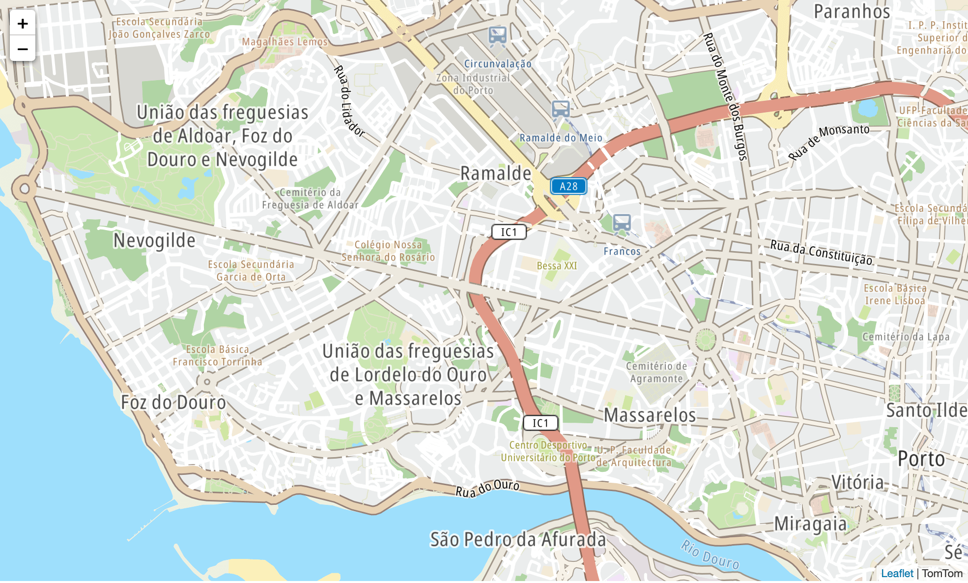

To add a polyline to the map, use the following code:

def polyline_to_list(polyline):
    """
    The polyline_to_list_lists function transforms the raw polyline to a list of tuples
    input: '[[-8.639847,41.159826],[-8.640351,41.159871]'
    output: [[41.159826, -8.639847],[41.159871, -8.640351]]
    """
    trip = json.loads(polyline) # json.loads converts the string to a list
    coordinates_list = [list(reversed(coordinates)) for coordinates in trip]
    # transform list (reverse values and put it in a list of lists)
    return coordinates_list

# Plot polyline on the map
polyline = polyline_to_list(df['POLYLINE'][1])
folium.PolyLine(polyline).add_to(TomTom_map)
TomTom_map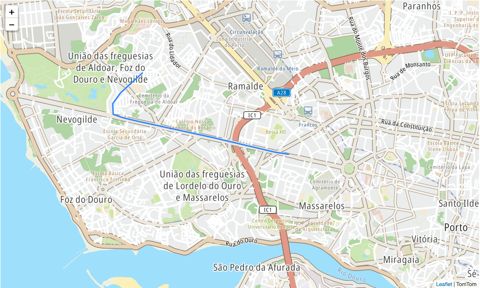

Step 4: How to use the TomTom Routing API

The first taxi trajectory in the dataset is now plotted on the map. Did this taxi driver take the fastest route? We can use the TomTom Routing API to find out.

Of course, traffic situations also influence the routes taken by taxi drivers. Fortunately, there is a way to account for that with the TomTom Routing API, by passing it a timestamp.

Let’s take a closer look at how it works. TomTom uses historic traffic to predict what the fastest route will be in the future. We do this by using temporal speed graphs called Speed Profiles.

For each road segment, we have a graph that shows the distribution of average speed (kmph) throughout the day. Provided we pass the correct day and time (e.g. Monday 16:05) to the Routing API, it will take into account the correct historic traffic distribution when calculating a route.

Convert UNIX time to ISO date

In order to be able to pass it to the API, we have to convert our UNIX timestamp to the similar weekday in the future, as we can only call the Routing API for current or future routes. We use the following function:

def convertUnixTimeToDate(timestamp):
    """
    The convertUnixTimeToDate function transforms a UNIX timestamp to a ISO861 dateTime format
    for a date in the future
    input: 1372636858
    output: '2024-05-3T00:00:58Z'
    """

    # Portugal is in UTC+0 time zone, first get the right time zone:
    UTC = tz.gettz('UTC')

    # Then convert our timestamp to the right format:
    timeTrip = datetime.datetime.fromtimestamp(timestamp,tz=UTC)
    weekday = timeTrip.strftime("%A") # get day of the week
    timeofday = timeTrip.strftime("%H:%M:%SZ") # get time of the day

    # Some hardcoded weekday dates in the future. Not the most elegant solution but fast:
    convertWeekdays = {
        "Monday":"2024-05-3T",
        "Tuesday":"2024-05-4T",
        "Wednesday":"2024-05-5T",
        "Thursday":"2024-05-6T",
        "Friday":"2024-05-7T",
        "Saturday":"2024-05-8T",
        "Sunday":"2024-05-9T"}

    routingTime = convertWeekdays[weekday] + timeofday

    return routingTime

Dealing with noisy GPS traces

The polylines in the Kaggle dataset are bit noisy. Fortunately, the TomTom Routing API has a route reconstruction option to deal with noisy GPS traces. By supplying supporting points as input to the Routing API, it can reconstruct a route which is matched to the TomTom map.

You can see an example in the image below:

In the next section, we will supply the Routing API with supporting points to ensure it calculates the duration for the correct trace.

Now that we are ready, let's call the TomTom Routing API

We define a function that lets us call the Routing API. As input, you provide it with a polyline from the Kaggle dataset, the corresponding UNIX departure time, your personal TomTom API key and whether you want to compute the taxi route or the fastest route.

def call_routing_api(polyline, departure_time, api_key=api_key, taxi_route=True):
    """
    Input is a polyline of a taxi route, a UNIX departure time, and whether to get the results for the taxi
    route or fastest route
    Output is the traffic delay in seconds, travel time of the route, route points from the Routing API and
    the full response from the API
    """

    coordinates_list = polyline_to_list(polyline) # transform polyline to list of tuples

    lat1, lon1 = coordinates_list[0] # origin coordinates of the trip
    lat2, lon2 = coordinates_list[-1] # destination coordinates of the trip

    # Set the URL for the Routing API
    routing_url = "https://api.tomtom.com/routing/1/calculateRoute/"
    url = str(routing_url + str(lat1) + ',' + str(lon1) + ':' + str(lat2) + ',' + str(lon2) +
    "/json?maxAlternatives=0&departAt=" + convertUnixTimeToDate(departure_time) +
    "&traffic=true&key=" + api_key)

    # Add support points for the route reconstruction:
    body = {"supportingPoints": []}

    if taxi_route == True:
        support_points = polyline_to_list(polyline) # use the whole polyline
        for point in support_points:
            body["supportingPoints"].append({"latitude": point[0],"longitude": point[1]})
    else:
        support_points = polyline_to_list(polyline)[-1] # use only the final coordinate
        body["supportingPoints"].append({"latitude": support_points[0],"longitude": support_points[1]})

    # Send the API call to TomTom:
    n = 0
    while True:
        n+=1
        try:
            response = requests.post(url,json=body)

            # Call was succesful"
            if response.status_code == 200:
                break

            # Call broke QPS limit, sleep for one second:
            elif response.status_code == 403:
                time.sleep(1)
        except:
            print("error", str(response.status_code))

        # Stop after 4 attempts:
        if n > 4:
            break
    # Return None if the call was not succesful
    if response.status_code == 200:
        response = response.json()

        delay = response['routes'][0]["summary"]['trafficDelayInSeconds']
        travel_time = response['routes'][0]["summary"]['travelTimeInSeconds']
        points = response['routes'][0]['legs'][0]['points']
        route_points = [[point['latitude'], point['longitude']] for point in points]

        return delay, travel_time, route_points, response
    else:
        return None, None, None, None

Step 5: Taxi trip analysis

The routing function is now ready to be used in our analysis. Let's start with checking the route we plotted earlier:

# First we calculate the travel time and route for the original taxi trip:
delay_taxi, travel_time_taxi, route_points_taxi, response_taxi = call_routing_api(df['POLYLINE'][1], df['TIMESTAMP'][1], taxi_route=True)

print("The taxi route will take you:", travel_time_taxi, 'seconds')

# Next we calculate the travel time and route for the fastest route:
delay_fastest, travel_time_fastest, route_points_fastest, response_fastest = call_routing_api(df['POLYLINE'][1], df['TIMESTAMP'][1], taxi_route=False)

print("The fastest route will take you:", travel_time_fastest, 'seconds')

The taxi route will take you: 657 seconds
The fastest route will take you: 657 seconds

The travel time is the same, let's also check the routes by plotting them on the map.

# Initialise TomTom map
TomTom_map = initialise_map(location=[41.164962,-8.656301], zoom=15)

# Plot the points of the original route on the map
polyline = polyline_to_list(df['POLYLINE'][1])
folium.PolyLine(polyline, color="blue", weight=2, opacity=1).add_to(TomTom_map)

# Plot the points of the original reconstructed route on the map
folium.PolyLine(route_points_taxi, color="black", weight=2, opacity=1).add_to(TomTom_map)

# Plot fastest route on the map
folium.PolyLine(route_points_fastest, color="red", weight=2, opacity=1).add_to(TomTom_map)

TomTom_map

It seems like this taxi driver was honest and took the fastest route, hooray!

Time to scale up

The previous example shows us the difference in seconds between the fastest route and the route that was taken by the taxi driver. The lower the average number, the more honest our taxi drivers are.

To answer the question, we posed at the beginning of the article, we will use a random sample of 1200 taxi trips. This will give us a good idea of whether taxi drivers in Porto take the faster route or not.

# retrieve 1200 random samples
random_sample = df.sample(1200, random_state=123)
random_sample = random_sample.reset_index().drop('index', axis=1) # reset index so we can iterate

# initialise dictionary in which we will store our results
results = {"Fastest_traveltime": [], "Taxi_traveltime": [],"Polyline" :[]}
# For each polyline in random_sample, call the call_routing_api function twice, once to retrieve the travel time
# for the fastest route and once for the travel time of the taxi route

for i in tqdm( range(len(random_sample)) ):
    if random_sample['POLYLINE'][i] != '[]': # check if polyline is not empty

    # travel time fastest route
    results['Fastest_traveltime'].append(
        call_routing_api(random_sample['POLYLINE'][i], random_sample['TIMESTAMP'][i], taxi_route=False)[1])

    # travel time taxi route
    results['Taxi_traveltime'].append(
        call_routing_api(random_sample['POLYLINE'][i], random_sample['TIMESTAMP'][i], taxi_route=True)[1])

    # add departurePoint to results:
    polyline = polyline_to_list(random_sample['POLYLINE'][i])
    results['Polyline'].append(polyline)
100.|██████████| 1200/1200 [13:34<00:00, 1.58it/s]

# save results as pandas dataframe
results = pd.DataFrame(results)

# calculate the difference in minutes between the two routes
results['Difference_min'] = (results['Taxi_traveltime'] - results['Fastest_traveltime']) / 60

# calculate the relative difference between the two routes
results['Relative_diff'] = (results['Taxi_traveltime'] - results['Fastest_traveltime']) / results['Fastest_traveltime']

# keep only the trips that are long enough to make a proper comparison
results = results[results['Fastest_traveltime'] > 60] # trips should take at least 1 minute

# display dataframe
results.head()

| | Fastest_traveltime | Taxi_traveltime | Polyline | Difference_min | Relative_diff | | --- | --- | --- | --- | --- | --- | | 0 | 1040 | 1351.0 | [[41.161815, -8.602632], [41.161914, -8.602533... | 5.183333 | 0.299038 | | 1 | 470 | 470.0 | [[41.161086, -8.604126], [41.161509, -8.603937... | 0.000000 | 0.000000 | | 2 | 560 | 679.0 | [[41.14602, -8.612442], [41.146452, -8.612208]... | 1.983333 | 0.212500 | | 3 | 520 | 555.0 | [[41.150637, -8.647785], [41.150727, -8.648802... | 0.583333 | 0.067308 | | 4 | 872 | 1033.0 | [[41.162436, -8.644959], [41.162481, -8.644986... | 2.683333 | 0.184633 |

print("Maximum relative difference is", round(max(results['Relative_diff']), 2))
Maximum relative difference is 11.74

A large number like this is of course not realistic. Apparently, some GPS traces are still too noisy causing these outliers. Let's filter them out:

# filter out outliers
results = results[results['Relative_diff'] < 2]

Final results

Now that we have our results, can we see what the mean difference in minutes is between the fastest route and the taxi route?

print("Mean:", np.mean(results['Difference_min']))
print("Standard deviation:", np.std(results['Difference_min']))
Mean: 2.5056110102843316
Standard deviation: 3.538457376554713
    

We can also plot the distribution of the difference in minutes and the relative difference, respectively.

# Plot histogram
difference_min = sorted(np.array(results['Difference_min']))
fig = plt.figure(figsize=(15,8))
plt.hist(difference_min, bins=15)
plt.title("Difference in minutes with the fastest route")
plt.xlabel("Minutes")
plt.ylabel('Counts')

# Plot histogram
difference_min = sorted(np.array(results['Relative_diff']))
fig = plt.figure(figsize=(15,8))
plt.hist(difference_min, bins=15)
plt.title("Relative difference with fastest route")
plt.xlabel("Relative difference")
plt.ylabel('Counts')

Another way to represent the data is by using percentiles.

# Get some percentiles of the relative difference
results['Relative_diff'].quantile([0.1, 0.23, 0.24, 0.5, 0.6, 0.75, 0.835, 0.9, 0.95, 0.98, 1])
0.100 0.000000
0.230 0.001009
0.240 0.004345
0.500 0.138331
0.600 0.199668
0.750 0.351191
0.835 0.491842
0.900 0.703618
0.950 0.941956
0.980 1.344909
1.000 1.970732
Name: Relative_diff, dtype: float64

From this we can conclude that although most taxi drivers are taking the fastest - or a similar - route (around 23%), there are still quite a lot of trips (16.5%) where taxi drivers take more than 50% longer than the calculated fastest route.

Step 6: Using Folium to Visualize the Data

First, we make a linear color scale, where green is no delay and red is more than 50% delay:

# Create a linear color scale
linear_color = cm.LinearColormap(['green', 'yellow', 'red'], vmin=0, vmax=0.5)
linear_color

We can plot taxi trip delays on the map.

The following plot will show the points where taxi trips started, with the corresponding delay they encountered along the way:

# Plot the starting point on the map
TomTom_map_bubble = initialise_map(api_key=api_key, location=[41.161178, -8.648490], zoom=13, style = "night")

for index, row in results[:1000].iterrows(): # limit number of data points plotted to 1000

    popup_string = "Relative delay = " + str(round(100* row["Relative_diff"], 1)) + "%"

    folium.Circle(
      location = row["Polyline"][0],
      popup= popup_string,
      radius=30,
      color=linear_color(row["Relative_diff"]), #get_color(row["Relative_diff"]),
      fill=True,
      ).add_to(TomTom_map_bubble)

TomTom_map_bubble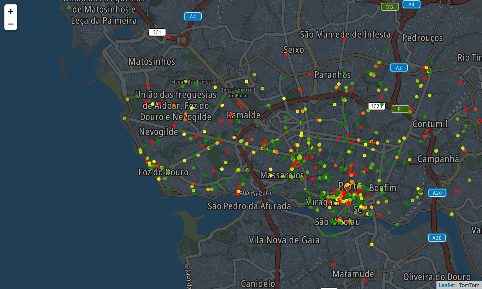

We can also make a (similar) plot that shows the taxi traces with their corresponding delay:

# On this map we visualize all the polylines of the taxi trips using the same color scheme
TomTom_map_lines = initialise_map(api_key=api_key, location=[41.161178, -8.648490], zoom=13, style = "night")
for index, row in results[:500].iterrows(): # limit number of polylines plotted to 500

    folium.PolyLine(row["Polyline"],
        color=linear_color(row["Relative_diff"]),
        weight=1.0,
        opacity=1.5
        ).add_to(TomTom_map_lines)

TomTom_map_lines 

Route planning saves time and money

Overall, we can conclude that:

1. Taxi trips would be 21% shorter if all taxis in Porto used TomTom navigation.

2. In 23% of the cases, your taxi driver will take the fastest or a similar route.

3. However, 40% of taxi trips will take more than 20% longer than the TomTom route.

Are taxi drivers taking a detour 40% of the time?

No. Taxi drivers are generally very knowledgeable about the cities they drive in and their experience allows them to outsmart traffic. While the analysis we’ve just performed allows us to draw conclusions, it is important to keep these factors in mind:

• The Kaggle taxi traces are quite noisy, which means that the GPS points recorded may deviate from reality and will not always be matched to the correct street. This means there is a margin of error in the results, and not all detours seemingly taken may be real.

• The taxi traces are dated: from 2013 and 2014. The analysis was done based on a map of 2019. As a result, there may be faster routes available today (e.g. due to new road infrastructure, new or improved traffic lights, new roundabouts, etc.) that did not exist at the time that the taxi rides took place.

• The speed profiles used in this analysis are a simplified version of reality and do not include traffic incidents. At the time that the taxi rides took place, there may have been road blockages or severe traffic jams – none of which have been taken into account in the analysis, but which may have forced the taxi driver to take a detour nevertheless.

You can find the TomTom Maps APIs documentation at to see what else is available. Our APIs cover everything from geocoding to points of interest (restaurants, hospitals, etc.), to solve the needs of developers and their customers alike.